Introduction: A New Era in Structural Biology

The last few years have seen a revolution in structural biology, driven by the breakneck speed of advances in artificial intelligence. This post is the first in a series where we will deconstruct the key architectures that have defined this new era. Our journey will take us from the deterministic brilliance of AlphaFold 2 to the generative power of modern diffusion models like Boltz-2.

To understand where the field is going, we must first build a deep appreciation for the foundation upon which it all stands.

In this first article, we focus entirely on AlphaFold 2, the model that solved one of biology’s 50-year-old grand challenges: the protein folding problem. We will move beyond a high-level overview to dissect its two-part engine:

• The Evoformer trunk, which established a rich, bidirectional dialogue between evolutionary data and a geometric hypothesis.
• The deterministic Structure Module, which used intricate, physically-inspired attention mechanisms to translate this hypothesis into a precise 3D structure.

By the end, you will have a solid, technically-grounded understanding of how AlphaFold 2 works, setting the stage for our exploration of the models that followed.

The Basics—Proteins, Residues, and Evolution

Before we dive in, let’s cover three foundational concepts.

Proteins and Residues
Think of a protein as a long, intricate necklace made of a specific sequence of beads. Each “bead” is an amino acid, which in this post is almost always called a residue. There are 20 common types of these residues, each with unique chemical properties.

The Protein Folding Problem
The central challenge of structural biology is that this 1D string of residues folds itself into a single, complex, and functional 3D shape. For 50 years, predicting this final 3D shape from only the 1D sequence of residues was a grand challenge in science. This is the problem AlphaFold 2 solved.

MSA (Multiple Sequence Alignment)
To get clues about the 3D shape, scientists look at the protein’s “evolutionary cousins” found in other species. An MSA is a massive alignment of these related sequences. Why is this important? If two residues are touching in the 3D structure, a mutation in one is often compensated by a matching mutation in the other across many “cousin” sequences. By finding these correlated pairs of mutations (a signal called co-evolution), the model gets powerful hints about which residues are close to each other in the final structure.

Long before diffusion models entered the mainstream for structural biology, AlphaFold 2[¹] achieved a watershed moment. When DeepMind presented their results at the CASP14 competition in late 2020, they didn’t just improve upon existing methods; they shattered all expectations, leaving the entire field of computational biology wondering how it was possible.[²]

When the paper and code were finally released, the “secret sauce” was revealed. It wasn’t a single, magical insight into protein folding, but rather a masterpiece of deep learning[³] engineering that fundamentally reinvented how to reason about protein structure. The computational heart of this masterpiece consists of two main engines working in concert: the Evoformer and the Structure Module.

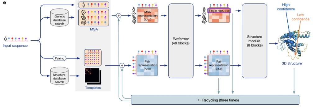Figure 1. The model is conceptually divided into three stages. First, input features are generated from the primary sequence, a Multiple Sequence Alignment (MSA), and optional structural templates. Second, the Evoformer block iteratively refines an MSA representation and a pair representation in a deep communication network. Finally, the Structure Module translates the refined representations into the final 3D atomic coordinates.

1. The Evoformer’s Engine: The Attention Mechanism

The Evoformer’s architecture is built on the now-ubiquitous transformer[⁴]. Its core computational tool is the attention mechanism, a powerful technique that allows the model to learn context by weighing the influence of different parts of the input data on each other (see Appendix of this blog series for a numeric walk-through[⁵]). When processing a specific residue, for example, it learns how much “attention” to pay to every other residue in the protein, allowing it to dynamically identify the most important relationships. For an excellent visual explanation of this concept, see Alammar[⁶].

1.1 Building the Blueprint: The Representations and Templates

The self-attention mechanism is a powerful tool, but for it to work on a problem as complex as protein structure, it needs data representations that are far richer than simple word embeddings. For years, the state-of-the-art approach was to take a Multiple Sequence Alignment (MSA) and distill its evolutionary information down into a single, static 2D contact map[⁷]. Methods would analyze the MSA to predict which pairs of residues were likely touching, and this map of contacts would then be fed as restraints to a separate structure-folding algorithm.[⁸]

AlphaFold 2’s paradigm shift was to avoid this premature distillation. Instead of collapsing the rich evolutionary data into a simple 2D map, it builds and refines two powerful representations in parallel, providing the perfect canvas for its attention-based Evoformer. Let’s look at how these representations are constructed.

1.1.1 The MSA Representation: A Detailed Evolutionary Profile

AlphaFold 2 first clusters the MSA. The model then processes a representation of size ($N_{seq}$ × $N_{res}$), where $N_{seq}$ is the total number of sequences in the stack (composed of both MSA cluster representatives and structural templates) and N_res is the number of residues.

The key is that for each residue in a representative sequence, the model starts with a rich, 49-dimensional input feature vector. To make this concrete, imagine the model is looking at residue 50 of a representative sequence, which is a Leucine (L). Its input vector would answer several questions simultaneously:

• What is this residue?
  A set of channels acts as a one-hot encoding, where the channel for “Leucine” is set to 1 and all others are 0.

• What is the local structural context? The Deletion Profile.
  Other input channels track a deletion profile from the MSA, answering the question: “Across all related sequences, how often is a residue missing at this spot?” This provides a powerful structural hint, as a high frequency of deletions suggests a flexible loop, while a low frequency points to the protein’s stable, conserved core.

• What is its evolutionary context?
  A large portion of the vector is dedicated to the cluster’s statistical profile. This profile summarizes all the sequences in that family branch, saying something like: “For position 50, Leucine appears 70% of the time, Isoleucine appears 20%, and Valine appears 5%.”

This 49-dimensional input vector is then processed by a linear layer to produce the internal MSA representation, which has 256 channels ($c_{m}=256$). This is the representation that is iteratively refined within the Evoformer.

1.1.2 The Pair Representation: The Geometric Blueprint

This is a square matrix of size ($N_{\text{res}} \times N_{\text{res}}$) with 128 channels ($c_{z}=128$) that evolves into a detailed geometric blueprint of the protein. It’s the model’s internal hypothesis about the 3D structure. It doesn’t start as a blank slate; the initial representation $z_{ij}$ is constructed from the primary sequence itself, seeding the model with fundamental information about residue identity and position. This is done in two steps:

1.1.2.1 Encoding Residue Pairs via Outer Sum

First, the model learns two separate 128-dimensional vector representations, $a_{i}$ and $b_{j}$, for each amino acid at positions $i$ and $j$. These are learned by passing the one-hot encoding of the amino acid type through two different linear layers. The initial pair information is then created by simply adding these vectors:

This operation creates a basic ($N_{\text{res}} \times N_{\text{res}}$) map where each entry is a 128-dimensional vector influenced by the specific amino acids at positions $i$ and $j$.

1.1.2.2 Encoding Relative Position

Next, the model explicitly injects information about the 1D sequence separation. It calculates the relative distance $d_{ij} = i - j$, which is clipped to a fixed window (e.g., between $-32$ and $+32$) and converted into a one-hot vector. This binary vector is then passed through another linear layer to create a dedicated 128-dimensional positional embedding, $p_{ij}$.

The final initial pair representation is the sum of these two components:

This initial grid is like digital graph paper, with basic 1D relationships sketched out. The job of the Evoformer is to enrich this grid, filling its 128 channels with sophisticated 3D information like residue-pair distances and orientations.

1.1.3 Structural Templates: A Powerful Head Start

The third, optional source of information comes from structural templates. If homologous structures[⁹] exist in the PDB, AlphaFold 2 leverages their known geometry not as a rigid scaffold, but as a set of powerful, editable hints. This information is integrated through two distinct and sophisticated pathways:

1.1.3.1 A 2D Geometric Hint for the Pair Representation

First, the model extracts key geometric features from each template, most notably a distogram[¹⁰]—a detailed map of distances between all pairs of residues. This collection of geometric data is then processed by its own dedicated “Template Pair Stack.” This stack refines the template information using a simplified version of the powerful triangular updates, a core mechanism of the Evoformer that we will deconstruct shortly.

The model then integrates this refined template data into its main geometric blueprint using a clever attention process. For every residue pair $(i, j)$, a specialized attention mechanism assesses the geometric hints provided by all available templates. It effectively asks a crucial question: “For this specific pair, which of my templates offers the most reliable geometric clue?” Based on the answer, it calculates a weighted average of the geometric information from all templates and adds this “consensus hint” directly to its own evolving blueprint. This process allows the model to intelligently fuse information, for instance, by trusting one template for a local helix while relying on another for the orientation of a distant domain.

1.1.3.2 A 1D “Advisor” for the MSA Representation

Second, in a particularly elegant move, the model extracts the known backbone torsion angles from the templates. These angles are embedded into a feature vector and then concatenated directly to the MSA representation as if they were additional sequences[¹¹]. This treats the template not as a static map, but as an expert participant in the evolutionary dialogue. By sitting alongside the other sequences, its structural information can directly bias the MSA attention mechanisms. For example, if a template’s torsion angles clearly define a beta-strand, it can encourage the MSA attention to focus on finding the long-range co-evolutionary signals that are characteristic of beta-sheet formation.

1.2 The Evoformer’s Work Cycle: A Refinement Loop

The Evoformer’s power comes from repeating a sophisticated block of operations 48 times. Each pass through this block represents one full cycle of the “dialogue” between the evolutionary and geometric representations.

Evoformer’s Dialogue—A Summary

The core magic of the Evoformer lies in its two-way communication stream, repeated over 48 cycles. Think of it as a feedback loop:

• Path 1 (MSA $\rightarrow$ Pairs): The model analyzes the evolutionary data (MSA) to find correlated mutations. It summarizes this evidence and sends it to the geometric blueprint (Pair Representation), saying: “Here are the residue pairs that are evolutionarily linked. You should probably move them closer together.”

• Path 2 (Pairs $\rightarrow$ MSA): The model then uses its current 3D hypothesis (Pair Representation) to guide its search through the evolutionary data. It tells the MSA attention mechanism: “I have strong geometric evidence that these two residues are close. Pay extra attention to any co-evolution signal between them, no matter how subtle.”

This cycle allows the model to build confidence by finding evidence that is consistent across both the evolutionary and geometric domains.

The goal is to use the attention tools to enrich both the MSA and Pair representations, making each one more accurate based on feedback from the other. A single cycle, or block, consists of three main stages: updating the MSA stack, updating the pair stack, and facilitating their communication.

1.2.1 Stage 1: Processing the Evolutionary Data (The MSA Stack)

The block first focuses on the MSA representation to extract and refine co-evolutionary signals. This is done with a specialized MSA-specific attention mechanism.

Axial Attention. To handle the massive ($N_{seq} \times N_{res}$) MSA matrix, the model doesn’t compute attention over all entries at once. Instead, it “factorizes” the attention into two much cheaper, sequential steps:

• Row-wise Gated Self-Attention. Performed independently for each sequence (row), this step allows the model to find relationships between residues within a single sequence.
• Column-wise Gated Self-Attention. Performed independently for each residue position (column), this step allows the model to compare the “evidence” from all the different evolutionary sequences for that specific position in the protein.

MSA Transition. After the attention steps, the MSA representation passes through an MSATransition layer. This is a standard point-wise, two-layer feed-forward network (MLP) applied to every vector in the MSA representation, allowing for more complex, non-linear features to be learned[¹²].

1.2.2 Stage 2: Enforcing Geometry (The Pair Stack)

The block now turns to the pair representation ($z$), the model’s geometric blueprint. At this stage, the blueprint might contain noise or local predictions that are not globally consistent. The goal of the Pair Stack is to refine this blueprint by enforcing geometric constraints across the entire structure. Its primary tool is a set of novel “triangular” operations. As detailed in Figure 2, these operations pass information through all possible residue triplets to ensure the final blueprint is physically plausible.

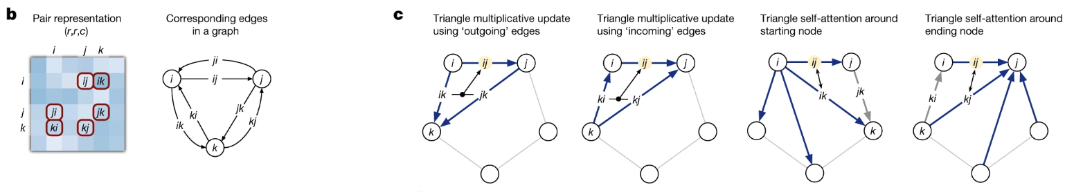
• Figure 2. The triangular operations at the heart of the Evoformer. The core idea is that information about the relationship between residues (i, k) and (k, j) provides strong evidence about the ‘closing’ edge of the triangle, (i, j). As shown in panel (c), the model enforces this geometric consistency using two distinct mechanisms: a gated multiplicative update and a more selective, bias-driven self-attention step, which are applied to all possible triangles.*

Triangular Multiplicative Update: Densifying the Geometric Graph.

This first operation acts as a fast, “brute-force” way to strengthen local geometric signals. It considers every possible intermediate residue $k$ for each pair $(i,j)$ and aggregates the evidence from all of them. As shown in the first two panels of Figure 2c, it combines information from the other two edges of the triangle. The process is gated to control the information flow:

1. It first computes an update vector by combining information from the other two edges in the triangle. For the “outgoing” update, the logic is:

   \[\text{update\_vector} = \sum_{k} \left( \text{Linear}(z_{ik}) \odot \text{Linear}(z_{jk}) \right)\]

2. It then computes a gate vector, $g_{ij} = \text{sigmoid}(\text{Linear}(z_{ij}))$, which acts as a dynamic filter based on the current state of the edge being updated.

3. Finally, the gated update is applied: $z_{ij} \mathrel{+}= g_{ij} \odot \text{update_vector}$.

By summing over all possible intermediate residues $k$, this mechanism efficiently ensures that the information in the pair representation is locally consistent and dense. The entire process is repeated symmetrically for “incoming” edges.

Triangular Self-Attention. While the multiplicative update is powerful, it treats all triangles equally. Triangular Self-Attention is the more sophisticated and arguably more critical operation, as it allows the model to be selective and propagate information over long distances. As visualized in the last two panels of Figure 2c, the representation for an edge (i, j) acts as a “query” to selectively gather information from other edges.

In simple terms, this mechanism allows the model to use a ‘buddy system’: it uses its knowledge about the relationship between residues A and C to intelligently refine its understanding of the relationship between A and B.

Let’s break down the “starting node” version into its key steps:

Let’s break down the “starting node” version into its key steps:

1. Project to Query, Key, Value.
   First, the model projects the pair representations into Query, Key, and Value vectors. For our query edge, we have $q_{ij} = \text{Linear}(z_{ij})$. For the edges it will attend to, we have $k_{ik} = \text{Linear}(z_{ik})$ and $v_{ik} = \text{Linear}(z_{ik})$.

2. Calculate Attention Score with Triangle Bias.
   For each potential interaction between edge $(i,j)$ and edge $(i,k)$, the model calculates a score. Crucially, this score includes a learned bias that comes directly from the triangle’s closing edge, $z_{jk}$: \(\text{score}_{ijk} = \frac{q_{ij} \cdot k_{ik}}{\sqrt{d_k}} + \text{Linear}(z_{jk})\) This allows the model to ask a sophisticated question: “How relevant is edge $(i,k)$ to my query $(i,j)$, given my current belief about the geometry of the third edge $(j,k)$?” This is what allows a confident local prediction in one part of the protein to rapidly inform a less confident prediction far away in the sequence.

3. Normalize and Gate.
   The scores for a given $i,j$ are passed through a softmax function over all possible nodes $k$ to get the final attention weights, $\alpha_{ijk}$. Separately, a gate vector, $g_{ij} = \text{sigmoid}(\text{Linear}(z_{ij}))$, is computed. The final output is the gated, weighted sum of all the value vectors: \(\text{output}_{ij} = g_{ij} \odot \sum_k \alpha_{ijk} v_{ik}\)

This entire process is then repeated symmetrically for the “ending node,” where edge $(i,j)$ attends to all edges ending at node $j$. The $O(N_{res}^3)$ complexity of these triangular operations makes them the primary computational bottleneck in AlphaFold 2, but they are essential for creating a globally consistent geometric blueprint.

Pair Transition.
Finally, the pair stack processing concludes with a PairTransition layer. This is a standard point-wise, two-layer feed-forward network (MLP) that is applied independently to each vector $z_{ij}$ in the pair representation[¹³]. This step allows the model to perform more complex transformations on the features for each pair, helping it to better process and integrate the rich information gathered from the preceding triangular updates.

1.2.3 Stage 3: The Bidirectional Dialogue (The Communication Hub)

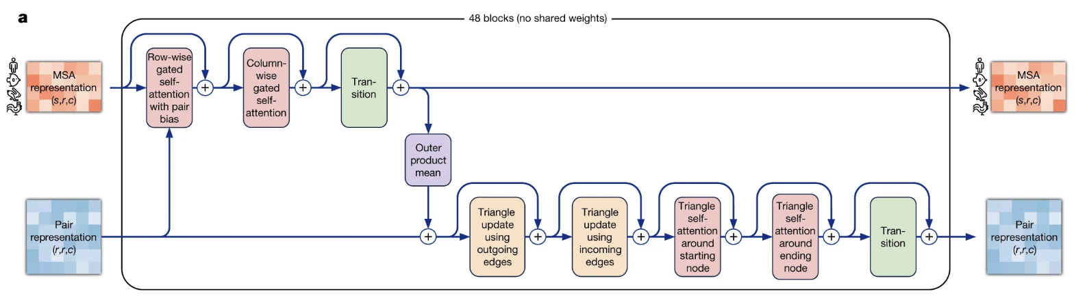Figure: The core logic of an AlphaFold2 Evoformer block. Information is exchanged between the 1D MSA representation and the 2D pair representation. The key innovation is the triangular self-attention mechanism within the pair representation, which enforces geometric consistency by reasoning about triplets of residues (i, j, k).

The MSA and Pair stacks don’t operate in isolation. The true genius of the Evoformer is how they are forced to communicate within each block, creating a virtuous cycle where a better evolutionary model informs the geometry, and a better geometric model informs the search for evolutionary clues. This dialogue happens through two dedicated pathways.

Path 1: From MSA to Pairs (The Outer Product Mean).
This is the primary pathway for co-evolutionary information to update the geometric hypothesis. The mechanism, called the OuterProductMean, effectively converts correlations found across the MSA’s sequences into updates for the pair representation.

For a given pair of residues $(i, j)$, the model takes the representation for residue $i$ and residue $j$ from every sequence $s$ in the MSA stack ($m_{si}$ and $m_{sj}$). It projects them through two different linear layers, calculates their outer product, and then averages these resulting matrices over all sequences. In pseudo-code:

This operation is powerful because if there is a consistent pattern or correlation between the features at positions $i$ and $j$ across many sequences, it will produce a strong, non-zero signal in the averaged matrix. This directly injects the statistical evidence from the entire MSA into the geometric blueprint, telling it which residue pairs are likely interacting.

Path 2: From Pairs to MSA (The Attention Bias)

This is the equally important reverse pathway, where the current geometric hypothesis guides the interpretation of the MSA. This happens subtly during the MSA row-wise attention step.

When the model calculates the attention score between residue $i$ and residue $j$ within a single sequence, it doesn’t just rely on comparing their query and key vectors. It adds a powerful bias that comes directly from the pair representation.

The effect is profound. If the pair representation, $z_{ij}$, already contains a strong belief that residues $i$ and $j$ are in close contact, the bias term will be large. This forces the MSA attention to focus on that pair, effectively telling the MSA module: “Pay close attention to the relationship between residues $i$ and $j$ in this sequence; I have a strong geometric reason to believe they are linked, so any co-evolutionary signal here is especially important.” This allows the geometric model to guide the search for subtle evolutionary signals that confirm or refine its own hypothesis.

2. The Structure Module: From Feature Maps to Atomic Coordinates

After 48 Evoformer iterations the network possesses two mature tensors: a per-residue feature vector $s_i$ (“single representation”) and a per-pair tensor $z_{ij}$ (“pair representation”). The Structure Module must now turn these high-level statistics into a concrete three-dimensional model. It does so through eight rounds of a custom transformer block called Invariant Point Attention (IPA)[¹⁴] followed by a small motion model, Backbone Update. The entire pipeline is differentiable[¹⁵].

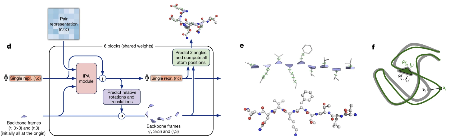Figure 4. The AlphaFold2 Structure Module. (d) The module takes the final single and pair representations and uses an Invariant Point Attention (IPA) module to iteratively update a set of local reference frames for each residue. (e) These local frames define the orientation of each amino acid. (f) The final output is a complete 3D structure, shown here superimposed on the ground truth.

The Structure Module’s Philosophy—Frames, Invariance, and Refinement

• Local Frames: Instead of predicting global coordinates, the model assigns a personal, local coordinate system (a “frame”) to each residue. It then learns to predict small rotations and translations to apply to each frame, unfolding the protein from a collapsed point. This makes the process robust to arbitrary global rotations.
• Invariant Point Attention (IPA): This custom attention mechanism decides which residues should interact by combining three signals: chemical/sequence similarity, the Evoformer’s 2D blueprint, and the current 3D proximity of the residues. Because it reasons about distances between points in local frames, its logic is “invariant” to the global orientation, respecting the physics of 3D space.
• Iterative Refinement: The final structure isn’t built in one shot. The IPA module iterates 8 times to refine the backbone. Furthermore, the entire prediction process is often “recycled” 3–4 times, where the model’s own previous output is used as an ultra-informative template to fix mistakes and improve accuracy in the next pass.

2.1 Local Frames Rather Than Global Coordinates

At the start of round 1, every residue $i$ is assigned an internal frame $T_{i} = (R_{i}, t_{i})$: a rotation matrix $R_{i} \in \mathrm{SO}(3)$ and an origin $t_{i} \in \mathbb{R}^{3}$. Think of this as giving each residue its own personal compass and position tracker. All frames are initialized to the same identity transformation in what the authors call a “black hole initialization”—the entire protein starts as a collapsed ball of overlapping atoms at the origin. This approach of operating in local frames has two key advantages:

1. Global rigid-body motions have no effect on distances measured within each frame, so the network never needs to learn arbitrary coordinate conventions.
2. Rotations and translations can be applied independently to each residue, allowing complex deformations to be accumulated over the eight cycles.

2.2 What Makes IPA “Invariant”?

Each residue advertises $K$ learnable query points $p_{i,k} \in \mathbb{R}^3$ that live in its local frame. These are like virtual “attachment points” that the residue learns to place on its surface to probe its environment. During attention, these points are converted to the global frame via:

This equation simply finds the location of each attachment point in the shared, ‘global’ space of the entire protein. The Euclidean distance $d_{ij, (k\ell)} = \left\lVert \tilde{p}{i, k} - \tilde{p}{j, \ell} \right\rVert_2$ is invariant to any simultaneous rotation or translation applied to all residues. This is the core insight: because the distance between two points is a physical constant regardless of viewpoint, an attention score built from this value respects the physics of 3D space without extra hand-crafting.

2.3 Scoring Who to Attend To

For each head $h$, the model decides how much attention residue $i$ should pay to residue $j$ by combining three distinct sources of evidence:

1. An Abstract Match: A standard attention score calculated from the query and key vectors of the single representation of the residues, asking: “Based on our learned chemical and sequential features, are we a good match?”
2. A Blueprint Bias: A powerful bias from the Evoformer’s final pair representation ($z_{ij}$), asking: “Does the 2D blueprint have a strong belief that we should be interacting?”
3. A 3D Proximity Score: A geometric score based on the distance between the residues’ virtual attachment points in the current 3D structure, asking: “Given our current positions in space, are we a good geometric fit?”

These three sources of evidence are then combined into a single, un-normalized attention score, calculated with learned coefficients ($w_{k\ell}^{(h)}$) and a length scale ($\sigma_{h}$):

2.4 Aggregating Messages

Softmax over $j$ produces attention weights $\alpha^{(h)}_{ij}$. Two distinct pieces of information, aggregated using these weights, are then passed back to residue $i$:

1. An abstract message, $m_i$, is calculated as a weighted sum of all other residues’ value vectors: \begin{equation} m_i = \sum_{h, j} \alpha^{(h)}_{ij} v^{(h)}_j \end{equation} This message updates the residue’s internal state, $s_i$, incorporating new chemical and sequential context based on the other residues to which the model just paid attention.

2. A geometric message—a set of averaged value points in the global frame—that is converted back to the local frame of $i$ through $T_{i}^{-1}$. This crucial step translates a global ‘group consensus’ on movement into a personal, actionable command for residue $i$, yielding a vector $\Delta x_{i}$ that captures where the residue “wants” to move.

2.5 Backbone Update

After the IPA block has updated the single representation $s_{i}$ with both abstract and geometric messages, the final vector is fed to a small MLP module called BackboneUpdate. This module’s job is to translate the abstract information in $s_{i}$ into a concrete movement command. This command consists of a translation vector, $\delta t_{i}$, and a 3D rotation vector, $\omega_{i}$.

The network predicts a simple 3D vector for the rotation because directly outputting the nine constrained values of a valid rotation matrix is very difficult for a neural network. Instead, it predicts an axis-angle vector ($\omega_{i}$), where the vector’s direction defines an axis of rotation and its length defines how much to rotate. The final rotation matrix, $\delta R_{i}$, is then generated using the exponential map[¹⁶], a standard function that reliably converts the simple vector command into a perfect $3 \times 3$ rotation matrix:

This command is a small, relative “nudge”—a slight turn and a slight shift. The frame is then updated by applying this nudge to its current state via composition:

Repeating IPA followed by Backbone Update eight times unfolds the chain into a well-packed backbone without ever measuring absolute orientation.

Why this Design Works

IPA gives the network three complementary signals when deciding if residues should be close: their biochemical compatibility (query–key term), the Evoformer’s experience (bias term), and the evidence of their current partial fold (distance term). The gating present in both the attention weights and the Backbone Update lets the model ignore unhelpful suggestions, preventing oscillations and speeding up convergence.

2.6 Side-Chain Placement

After the backbone has settled, a final set of MLP heads predicts the side-chain conformations. AlphaFold 2 does this elegantly by treating side chains not as individual atoms, but as a series of connected rigid groups. For each residue, the network uses the final single representation ($s_{i}$) to predict up to four torsion angles (${\chi_{1}, \ldots, \chi_{4}}$) that orient these rigid groups. To handle the circular nature of angles, the network actually predicts the sine and cosine of each angle ($\sin \chi_{n}, \cos \chi_{n}$) rather than the angle itself, which makes the loss function smooth. A particularly clever feature is how the loss function handles symmetric residues (like Tyrosine or Aspartate); it allows the network to be correct if it predicts either the true torsion angle or one that is rotated by 180 degrees, as both are physically equivalent.

Once these angles are predicted, all heavy side-chain atoms are placed sequentially using standard, idealized bond lengths and angles and conditionally relaxed[¹⁷]. Because this entire process is part of the differentiable computational graph, the model can be trained end-to-end; for example, a clash between two distal atoms can send a gradient signal all the way back to adjust the responsible torsion angle predictions.

3. The Training Objective: A Symphony of Losses

Measuring Success—Key Metrics & Loss Functions

• RMSD (Root Mean Square Deviation)
  The classic way to measure the similarity between two 3D structures. You optimally superimpose the predicted structure onto the true one and then calculate the average distance between their corresponding atoms. A lower RMSD means a better prediction.

• FAPE (Frame Aligned Point Error)
  AlphaFold 2’s primary loss function and a clever improvement over RMSD. Instead of one global superposition, FAPE measures the error of all atoms from the perspective of every single residue’s local frame. This heavily penalizes local errors—like incorrect bond angles—that RMSD might miss. It effectively asks for every residue: “From my point of view, are all the other atoms where they should be?”

• Distogram (Distance Histogram)
  A 2D plot where the pixel at position $(i, j)$ isn’t a single distance, but a full probability distribution across a set of distance “bins.” The distogram loss forces the Evoformer’s Pair Representation to learn this detailed geometric information.

A neural network as complex as AlphaFold 2 cannot be trained by optimizing a single, simple objective. The genius of the model lies not only in its architecture but also in its carefully crafted loss function, which is a weighted sum of several distinct components. This multi-faceted objective ensures that every part of the network learns its specific task effectively.

The main loss is the Frame Aligned Point Error (FAPE), which measures the accuracy of the final 3D coordinates. To ensure all parts of the model are learning correctly, several “auxiliary” losses provide richer supervision:

• Distogram Loss:
  The refined pair representation in the Evoformer is used to predict a distogram. This prediction is compared against the true distogram from the experimental structure. This loss ensures that the Evoformer’s geometric reasoning is accurate even before a 3D structure is built, providing a strong intermediate supervisory signal.

• MSA Masking Loss:
  In a technique inspired by language models like BERT, the model is given an MSA where some of the amino acids have been randomly hidden or “masked”. The model’s task is to predict the identity of these masked amino acids. This forces the Evoformer to learn the deep statistical ‘grammar’ of protein evolution, strengthening its understanding of co-evolutionary patterns.

• Predicted Confidence Metrics:
  AlphaFold 2 doesn’t just predict a structure; it predicts its own accuracy by generating a suite of confidence scores. These include the per-residue pLDDT to assess local quality, the Predicted Aligned Error (PAE) to judge domain packing, and the pTM-score to estimate the quality of the overall global fold. Training the model to predict its own errors is crucial for real-world utility, as it tells scientists when and how much to trust the output.

By combining these different objectives, the model is trained to simultaneously understand evolutionary relationships (MSA masking), reason about 2D geometry (distogram), build accurate 3D structures (FAPE), and assess its own work using its internal confidence scores. This symphony of losses is a key reason for its remarkable accuracy.

In a Nutshell: AlphaFold 2’s Key Innovations

Before we conclude, let’s summarize the core engineering breakthroughs that made AlphaFold 2’s success possible:

• Co-evolving Representations: Instead of a simple pipeline, the model refines an evolutionary hypothesis (MSA Representation) and a geometric one (Pair Representation) in parallel, forcing them to agree through a rich, bidirectional dialogue.

• Triangular Self-Attention: The critical innovation within the Evoformer. It enforces the geometric logic that if A is near B, and B is near C, then A and C must also have a constrained relationship, allowing local information to propagate globally.

• Invariant Point Attention (IPA): The engine of the Structure Module. By reasoning about distances in each residue’s local coordinate system (“frame”), it builds the 3D structure in a way that is robust to global rotations and translations, respecting the physics of 3D space.

• End-to-End Differentiable Training: The entire system, from input processing to the final 3D coordinates, is trained as a single network with a sophisticated set of loss functions (like FAPE), allowing every part of the model to learn directly from errors in the final structure.

A Summary of the Revolution

Ultimately, the genius of AlphaFold 2 lies in its integrated design. It doesn’t treat protein structure prediction as a simple pipeline, but as a holistic reasoning problem. The Evoformer creates a rich, context-aware blueprint by forcing a deep dialogue between evolutionary data and a geometric hypothesis. The Structure Module then uses a physically-inspired, equivariant attention mechanism to translate this abstract blueprint into a precise atomic model. This end-to-end philosophy, guided by a symphony of carefully chosen loss functions, is what allowed AlphaFold 2 to not just advance the field, but to fundamentally redefine what was thought possible.

References